网络最大流
任意一条网络流边可以描述为$x=(u,v,cap,flow)$。其中$u$为边的起点,$v$为边的终点,$cap$为流量限制,$flow$为当前流量……
网络流简介 (来自OI Wiki)
一 基础内容
任意一条网络流边可以描述为$x=(u,v,cap,flow)$。其中$u$为边的起点,$v$为边的终点,$cap$为流量限制,$flow$为当前流量。
- 反向边:对于任意一条有向边$e=(i,j,cap,flow)$,定义$e’=(j,i,0,-flow)$ 为它的反向边。注意,反向边在网络流图中是不真实存在的,它其实是一个反悔机制,因此它的流量限制为$0$。定义反向边的当前流量与其对应的正向边的当前流量互为相反数。
反向边图解,图片来自网络: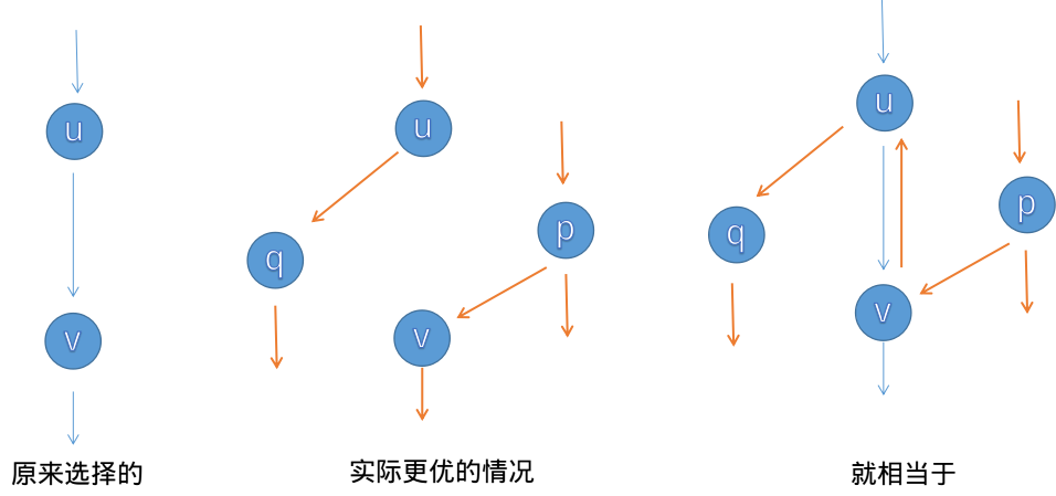
图中,选择$u\to v$和$p\to v\to u\to q$两条增广路径,实际上等同于选择$u\to q$和$p\to v$两条增广路径。因为路径$u\to v$和它的反向边$v\to u$的流量之和总为$0$,同时被选中,则意味着这条边对实际流量其实是没有贡献的(这两条边的贡献等于流量之和,等于$0$)。实际上就变成了这两条边同时不被选中。
残量网络:对于图上的任意一条边(包括反向边),定义它们的流量限制与当前流量之差为其残量。一张网络流图上所有边的残量构成残量网络。
增广路:一条从原点($s$)到汇点($t$)的路径,并且这条路径上每条边(包括反向边)的残量均大于$0$。设$f_i$为这条路上最小的残量,那么这条增广路可以使得当前流量增加$f_i$。
增广路定理:一张网络流图的流量达到最大流当且仅当残量网络中不存在增广路。
最大流最小割定理:一张网络流图的最大流永远等于该图的最小割的总容量(蒟蒻的我不会证明)。对于割的定义,可以参考割点。
二 Edmond Karp算法
1 流程
于是我们可以得出最朴素的最大流算法(Edmond Karp,EK算法)。
从原点开始,每次找一条到汇点的增广路径,并进行一次增广。
从原点出发向汇点搜索,设$m_i$为$s\to i$这条路上的最小残量$i$,$cap_e$为当前入边($e$)的流量限制,$flow_e$为当前入边的当前流量,可以得到递推式如下:
$$ m_i = \min m_j,cap_e-flow_e | e=(j,i),e \in E $$
每次到达汇点,将答案增广$m_t$,一直到残量网络中不存在增广路。于是就可以达到最大流。
注意反向边的储存。边表存图时,定义正向边编号为偶数,它的下一条边就是它的反向边。编号从$0$开始,则$i \text{xor} 1$总为$i$的对应边(正向边对应到反向,反向边对应到正向)。
2 实现
1 |
|
三 Dinic算法
在稠密图中,dinic算法的复杂度要比EK高到不知道哪里去了。
1 思想
dinic的主要思想是把一张网络流图分层,每次只往更深一层寻找增广路,以避免在同一层中绕圈子(这多半是无意义的)。
每当分层图中找不到增广路,这意味着当前图中至少有一条边的流量已经达到限制。也就是说这条边“断了”。而一条断了的边会改变图的分层情况,所以这时重新分层,并继续寻找增广路。
直到图上找不到一条$s\to t$的可行路径。也就是说所有道路都断了。此时会在图上会表现为找不到汇点的所在层级,因为根本没有到达汇点。说的更透彻一点,此时实际上是最小割被完全切断(最大流最小割定理)。
使用bfs完成图的分层,利用dfs寻找增广路径。
2 实现
1 |
|
3 优化
3-1 多路增广
上文中的代码一次搜索仅找出一条增广路,这样可能会在搜索时走很多重复的道路,造成一些常数负担。
所以每次在一条路上增广时,同时寻找多条增广路,直到干路的最小残量被用完或到达汇点时为止。这样可以避免重复走一条干路。
也就是说,一次dfs搜索所有的增广路。
3-2 当前弧优化
多路增广后,一条仍有残量却已经被增广的边是不可能继续被增广的,因为它所有的增广可能性已经被全部枚举了。所以继续dfs时,不需要再考虑这些边。所以设$cur_i$为新的边表表头,即以$i$为起点且没有被增广过的第一条边的编号,每次增广后更新$cur_i$即可。
注意,每次重新构造分层图后,$cur_i$需复原,因为此时对于 任意一条边 的 任意一种增广可能性 都没有考虑。
3-3 实现
1 |
|